The Commodity-by-Industry Approach

Until now we have assumed that every sector is uniquely associated to a good: steel is produced only by the steel producing sector, and the steel producing sector produces nothing but steel.

Let us assume there exist n industries which use and make m commodities. The m ? n Use matrix U (also called the absorption or input matrix) describes how much each industry purchases (that is, uses) of each commodity. The n ? m Make matrix V (also called the output matrix) represents how much each industry sells (that is, makes) of each commodity. These matrices are expressed in value terms, like matrix Z.

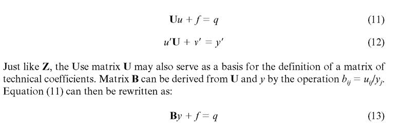
The interpretation of these matrices is straightforward. Let us begin with the Use matrix, which is of the commodities-by-industries type. If we sum all the purchases of commodity i by the m industries and add to that the final demand f for this commodity, we obtain the total output q_i of commodity i (in value terms). By contrast, if we sum all the purchases of commodities by industry j and add to that the value added v_j created in this industry, we obtain the total output y_j of industry j. In an obvious matrix notation, this means:

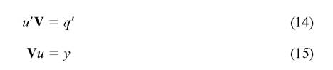
The Make matrix, on the other hand, is of the industries-by-commodities type. Instead of (11) and (12) we therefore have:

id="Picutre 70" class="lazyload" data-src="/files/uch_group31/uch_pgroup24/uch_uch7226/image/image070.jpg">

Equation (16) allows us to transform total commodity outputs into total industry outputs, and equation (17) to do the opposite.

If we use (16) in conjunction with (13) we arrive at the following relation between commodity outputs and final demand:

The matrix (I - BD)^-1 is called a commodity-by-commodity total requirements matrix. It plays a role similar to the Leontief inverse in (4). If the number of commodities is equal to the number of industries, and if matrix C happens to be invertible, another expression can be obtained which links commodity outputs to final demand. In fact, in that case we can use (17) in conjunction with (13) to arrive at:

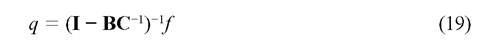
The matrix (I - BC^-1)^-1 is also called a commodity-by-commodity total requirements matrix.

We therefore have two matrices which are akin to the technical coefficients matrix A in the basic input-output model: matrix BD and matrix BC^-1. The first embodies the so-called industry-technology assumption. According to this inter­pretation, all commodities produced in a given industry have an identical input structure, equal to the corresponding column of matrix B. The second embodies the commodity-technology assumption. The interpretation here is that irrespective of the industry in which it is produced, a commodity is always produced with the same input structure.

The commodity-by-industry approach has been introduced by Richard Stone (1913­1991) and his collaborators. It provides a solid framework to connect input-output analysis to systems of national accounting. In 1968 the United Nations proposed the approach as a standard for data collection and presentation. This is now known as the United Nations System of National Accounts (UNSNA or simply SNA), of which the latest version was issued in 2008. The European System of Accounts (ESA), of which the most recent version dates from 2010, is to a large extent the same.

One of the problems that may, and often will, occur if one adopts the commodity­technology assumption, is the occurrence of negative elements in the technical coef­ficients matrix BC^-1. (Under the industry-technology assumption negative coefficients never occur.) Negative coefficients clearly have no sensible economic meaning. One solu­tion of the problem consists of replacing the negative elements, which tend to be small, by zeroes. A more radical solution is to abandon the commodity-technology assumption altogether.