Area, Data, and Statistical Model
The dataset is based on family reconstitutions carried out within the Scandian Demographic Database7 for nine parishes in western Scandia in southern Sweden. The sample used in this paper consists of four of these nine parishes: Hog, Kavlinge, Halmstad, and Sirekopinge.
The social structures of the parishes varied somewhat. Hog and Kavlinge were dominated by freeholders and tenants on crown land, a group rather similar to the freeholders regarding its social characteristics, while Halmstad and Sirekopinge were totally dominated by tenants on noble land (see Bengtsson and Dribe 1997; Dribe 2000). In addition to the peasant group, the parishes also hosted various landless and semi-landless groups, dependent on working for others to cover the subsistence needs of the family. In this chapter we will focus our attention on the landless and the semi-landless. Table 14.1 shows the social status of family heads in the four parishes. The peasant group has been subdivided according to type of land (freehold/crown land and noble land) and the productive potential of the landholding measured in maantal': The dividing line chosen—1/16 of a mantal—was the minimal amount of land required in the beginning of the nineteenth century to be considered as a landed peasant (besuttenhetsgrans) and it corresponded roughly to 15 acres in Scandia at that time (Sommarin 1939: 23, 29). As Table 14.1 clearly shows, the number of smallholders increased over the nineteenth century especially on freehold and crown land, implying that the proportion of peasants having landholdings below the minimum requirement increased, which serves to indicate the increased social differentiationTable 14.1 Social structure of family heads in the four parishes, 1766—1895 (in %)
| Social group | 1766-1815 | 1815-65 | 1865-95 |
| Higher occupations/nobil- ity | 1 | 1 | 1 |
| Landed peasant | |||
| Freeholders/crown ten- ants>1∕16 | 13 | 13 | 13 |
| Noble tenants>1∕16 | 25 | 12 | 2 |
| Semi-landless groups | |||
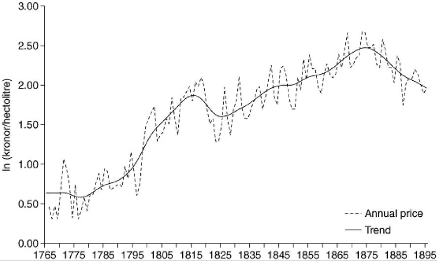
| Freeholders/crown ten- antsover time. We will use the price of rye in the analysis below as an indicator of economic fluctuations, but it can probably be seen as a more general indicator, which is not highly dependent on the actual mix of different crops in consumption and production. However, we lack data for long periods of time for some commodities of increasing importance, such as potatoes, animal products, housing, clothing, etc. Although we can expect that they became more important in the family budgets over time, even in the later part of the nineteenth century a large proportion of the food budget was spent on grain (Myrdal 1933). Thus, we believe that the fluctuations in grain prices were of great importance to rural families throughout all three phases of the whole period, and that they will therefore serve as rather good indicators of the economic situation of families, in particular of the landless. We also lack data on nominal wages at, or below, county level for the first period. Until the 1850s and the 1860s nominal wages were constant for long periods of time, implying that real wages, in the short term, mainly reflected grain price fluctuations. As was discussed previously, real wages, as measured by nominal wages deflated by the price of rye, stayed quite constant in Malmohus County until the mid-1860s and then increased steadily for the rest of the century (see Figure 14.1 above). In the short-run real wages show considerable variation, mostly due to variation in the rye price. Since our prime concern in this chapter is with the demographic response to short-term economic fluctuations, it makes sense to use the rye price as an indicator of economic stress. Figure 14.4 shows the logarithms of rye prices (actual values and Hodrick- Prescott trend) at the local level in the area under study.10 Clearly, there is a long-term trend in the price development, as well as medium-term cycles. It is not within the scope of the present study to analyse these trends and cycles. In order to picture the short-term fluctuations, we need to de-trend the series by subtracting the Hodrick-Prescott trend11 from the logged actual values. These detrended series are used in estimating the multivariate models below.Traditionally, particularly in aggregate studies, grain prices have often been used as proxies for harvest outcome, so that high grain prices reflect a bad harvest and low food supply, leading to increased mortality, delayed marriages, etc. However, when doing micro studies on small communities, the relationship between local harvest outcome and grain prices can be expected to have been rather weak, since a number of other factors become more important, such as trade, different external factors, the harvest outcome outside the region, etc. A comparison of grain prices and harvest outcome in western Scandia also corroborates this expectation; Figure 14.4 Natural log local rye prices (actual values and HP-trend), 1766/70-1891/95
Source. Bengtsson and Dribe 1997. there is only a very weak relationship between local harvest outcome and grain prices in the region.12 In times of a local harvest failure, grain could be bought from other regions, thereby smoothing prices. Similarly, severe harvest failures in other regions or other exogenous events could drive up local grain prices, without changes in the local harvest outcome. This implies that the grain price can only serve as a very poor indicator of the local harvest outcome. Instead, local grain prices must be seen as determined mainly exogenously. Ideally, we should include both the local harvest outcome and grain price in the analysis. For shorter periods of time this is also possible and has shown to be fruitful in the analysis of migration (Dribe 2000, 2003a). For the long period of time analysed here, however, this has not been possible, so we have limited the analysis to grain prices. For the landless and the semi-landless groups studied here, rising grain prices can be expected to have lowered the real wages, provided that they were paid money wages and that they were dependent on the market for their consumption. We know that they were often paid partly in money and partly in kind (e.g. Granlund 1944), but even in cases where they were paid in kind, the wage could be denoted in money and then converted into grain using the market price sales which implies that also payments in kind were negatively affected by high prices of grain. Hence, it is probably safe to assume that completely landless labourers were negatively affected by high grain prices.In estimating the models in the empirical analysis we use combined time-series and event-history analysis, which makes it possible to run regressions on the change of life status, that is, dying or giving birth to a child, measuring the effects of different explanatory variables (or covariates) on the hazard of the event. More specifically, we use the Cox proportional hazards model, which is distinguished from other proportional hazards models by not requiring any specification of the underlying hazard function with time varying external (community) covariates (Cox 1972; see also Collett 1994). The main interest in this case is to estimate the impact of different covariates on the hazard of the event.13 The model applied to mortality can be written as:
where h(a) is the hazard of the event for the ith individual at age a; h0(a) is the ‘baseline hazard', that is, the hazard function for an individual having the value zero on all covariates; β is the vector of parameters for the individual covariates X1 that are estimated; and γ is the parameter for the external time varying covariate Z(t). In the fertility analysis, we use time since last birth as the duration time (a) instead of age. In discussing the results below, relative hazards (or hazard ratios) are used as measures of the difference between groups with different values on the covariates. The relative hazards are the difference in the hazard of the event for the group under consideration, relative to the reference category. A value of 1.50 implies that the hazard of the event of interest in the group is 50% higher than in the reference category, while a figure of 0.50 implies that the hazard is 50% (or half) of the hazard in the reference category. The aggregated economic indicator (de-trended values of natural log rye price) is included in the regressions as a communal or external covariate (e.g. Bengtsson 1993), which means that the aggregate economic information is used as a time-varying covariate common to all individuals in the risk set at each point in calendar time. We show the mortality response to a 10% increase in prices in the tables, which was a modest price change during this period. The increase was higher than 120% in no fewer than fourteen years during this period. 5. More on the topic Area, Data, and Statistical Model: | |||