Monetarist Transitional Dynamics
Monetarist orthodoxy is not conclusively defined without reference to important works on the dynamics of the modified quantity theory. Friedman is again pivotal (see Friedman 1968, 1974, 1977).
The horizon of his short-run, policy-oriented quantity theory also includes the transitional dynamics towards a unique steady-state equilibrium. Monetary orthodoxy introduces transitional dynamics as a disequilibrium process (monetary nonneutrality). At the core of the theory is the assumption of adaptive expectations, that is, expected inflation is a weighted average of all current and past realized inflation rates. Even though the representative agent is not irrational (not subject to money illusion), he must “learn” to improve his forecast. Expectations are sluggish, because learning takes time. Accordingly, the speed of convergence depends on the persistence of past experience. In case only last period’s experience matters, inflation expectations are given by:
where πet denotes next period inflation rate currently expected, and λ gives the elasticity of expectations. Changes in the stance of monetary policy always come by surprise and are, therefore, non-neutral.
During the convergence process, the demand for money is predominantly determined by permanent income and inflation expectations. As a proxy for the steady-state wealth level, permanent income is thought to stabilize the money demand function. Of equal importance is the role of inflation expectations. Nothing in the Tract impressed Friedman more than Keynes’s “excellent and explicit discussion of inflation as a tax and of the [negative] effect of the tax on the quantity of real balances demanded” (Friedman 1974: 171). He was well aware that Keynes anticipated the Cagan model, which is a foundational contribution to monetarist orthodoxy (Cagan 1956).
Here, inflation expectations may account for bubbles (dynamic instability). Monetary policy is advised to rule out such explosive paths (hyperinflations) by committing to non-accelerating moneysupply rules.Permanent income is of minor importance in the neighbourhood of a steady-state equilibrium of a stable real economy. It does no harm to set the steady-state real growth rate equal to zero. Then, for the dynamic version of the quantity equa
tion is taken to yield the growth rate of nominal income:

where dotted lower case letter variables denote the percentage growth rates of the upper case letter variables, respectively. Note that growth of nominal income, given by U, is a separate variable. Furthermore, given that money supply is supposed to have an immediate impact on nominal income (as shown above), all variables are indexed with respect to the same time period. This is the monetarist theory of nominal income beyond the very short run.
To distinguish between the impact of money supply on transitional real-income growth and on inflation, Friedman introduced his variant of the Phillips curve relationship. Prior to Friedman (1968) and Phelps (1967), the Phillips curve implied a relationship between wage-driven inflation and an excess demand on the labour market. It was understood to explain inflation as disequilibrium phenomena: an excess demand (supply) for commodities translates into an excess demand for labour (involuntary unemployment), driving up (down) the nominal wage rate and - via mark-up pricing - the price level (for example, Lipsey 1960). Friedman rejected this early Phillips curve on the ground that it involves money illusion. Wage setters remain on their short-run labour supply curves, meaning that firms have to pay higher real wages to buy additional labour force.
This results in the monetarist or expectations-augmented Phillips curve:
where i denotes the elasticity of labour supply, w is wage inflation, u the actual unemployment rate, and u* the potentially inefficient steady-state rate of unemployment (due to labour market frictions of any type). Friedman’s controversial notion of the “natural rate of unemployment” is basically “the equilibrium reached by labor markets unaided and undistorted by governmental fine tuning” (Tobin 1972: 2).
Nominal wages were assumed to be more sluggish than commodity prices, such that rational wage setters must involve inflation expectations to protect their real claims. Given marginal productivity pricing in a competitive economy, there exists - for any given level of actual income - a close relationship between nominal wage growth and realized inflation. Let us assume that wt = πt. Substitution and rearrangement yield the Lucas-Rapping “surprise” function (Lucas and Rapping 1969), a cornerstone of monetarism:

summarizing one of the most important propositions of monetarism: deviations of unemployment from its natural level occur only in case of unanticipated inflation rates. To “stimulate the economy”, inflation must rise by surprise. Solving for realized inflation then gives:

introducing inflation expectations as a shift variable. Finally, transitional real-income growth is trivially given by:
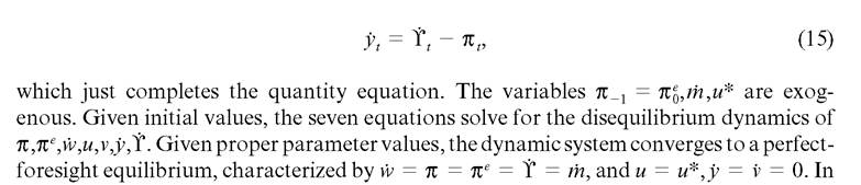
the steady state, nominal variables grow at the same constant rate determined by monetary policy. Furthermore, the classical dichotomy prevails in long-run equilibrium (the quantity prediction).
Augmenting the Phillips curve with expectations suggests that there exists no long-run trade-off between inflation and unemployment, since the curve shifts as soon as wage setters start to learn the money growth rate.Assume that a monetary authority decides to realize higher money supply growth. According to equation (11), the growth rate of nominal income immediately adjusts (the money-supply theory of nominal income). Given the actual inflation rate, equations (13)
and (15) suggest that the monetary impulse immediately induces output growth, thereby pushing the unemployment rate below its natural level. The monetarist disequilibrium dynamics display monetary non-neutrality. Realized inflation rises from the onset, due to an increasingly overheating labour market (equation 14). According to (10), they subsequently learn the stance of monetary policy; expectations catch up successively.
The velocity of money increases due to the eroding base of the expected inflation tax on real balances. This amplifies the monetary impulse: during the “early” stages of the transition, nominal and real incomes grow at a faster rate than money supply. The nonaccelerating money supply path rules out the explosive solutions. Note that the real wage rate is pro-cyclical in Friedman’s analysis, which is not confirmed by the facts.
The fame of the dynamic monetarist model is based on its ability to predict “stagflation”, a period of high inflation and low growth. Old variants of the Phillips curve (pure cost-push/demand-pull inflation explanations) suggested a persistent and exploitable trade-off between inflation and unemployment. The US stagflation during the 1970s could not be predicted by the “Keynesian” workhorse models. This was the momentum for the monetarist school, because stagflation is the predicted response to a monetary impulse during the late stages of the transition process. Because the early phase of the monetarist transition is one of “bamboozlement” (Tobin 1972), its late phase, when expected and realized inflation are already close, is a hangover.
Given equation (15), a convergent inflation process suggests decreasing real growth (stagflation). The role of the monetarist Phillips curve is decisive: the convergence is driven by its successive shifts during the learning process. In turn, the assumption underlying the expectations- augmented Phillips curve is the absence of money illusion.Rationality of the private sector is the key to Friedman’s dynamic analysis. Irrational behaviour, according to Friedman, cannot survive in a competitive market (Friedman 1953b: 22-3). As animal spirits and other irrationality are driven out by the impersonal market selection process, the observed amplitude of the business cycle must be largely due to policy failures. Friedman and the monetarists, of course, admitted that real and nominal variables are prone to demand and supply shocks. Yet, monetarism is founded on the presumption of a stochastically stable economy (like much of contemporary macroeconomics). This leaves little room for governmental fine-tuning.
Even worse, because fine-tuning works only with “long and variable lags”, discretionary monetary policy is highly pro-cyclical, even if well intended. Because money-supply management is highly effective, so much that there is nothing left for fiscal policy, central banks represent a permanent source of danger. A socially efficient solution, according to Friedman’s A Program for Monetary Stability (1960), would be to fire the money managers, and to replace them by a computer, programmed to increase the monetary base each month at a steady percentage rate (see also Simons 1936). Of course, the so-called “k-percent rule” is an extreme example. Monetarism usually prescribes nominal-income rules, that is, rules that counteract velocity shocks (see McCallum 1981). Friedman’s rule is illuminating, because it carries to extremes the spirit of monetarist orthodoxy.